| RESULTS |
| PS123 and simulated yield |
| PS123 model gave best result with 213 Julian planting date but model performance was poor with other planting date that was also used in the site. Therefore, the planting date best in the study site with this sets of climatic and crop data could be 213 Julian day. Further, model is well performed with different degree of salinity and maize yield is severely affected with salinity level beyond 8 dS/m in most soil units which is supported by several studies in different parts of the world. The result shows clay loam texture soil gives higher and less affected with soil salinity. It could be the effect of higher CEC and water holding capacity of the soil that delays in stress. |
| The model was tried to simulate the yield of cassava and rice with default crop parameters by changing total heat requirement and planting time. It simulates the cassava yield that is low but it did not performed well with rice. Since crop parameters vary from location to location that may lead to this result. Therefore, true site specific crop parameters could simulate reliable results. |
| Some selected measured soil salinity and fertility variables (EC, pH, CEC and OM) were used to estimate their variation in geopedologic units at �relief type� and at �landscape� levels, and also their spatial variation and dependency to estimate the area affected by salinity. Soil salinity and soil fertility varied significantly within and between geopedologic units at �relief type� and �landscape� levels (see table 2). Moving average gave best interpolation result in salinity and fertility modelling. PS123 simulates crop yield that correlates significantly with farmers yield (see table 1. ). This was not true for the case of CropSyst. Both models simulate crop yield with different degree of salinity (sensitivity analysis). Now a days, the development of GIS and remote sensing based models are used in various fields of studies. The GIS and remote sensing tools and techniques are commonly applied in natural resources management. These were also applied in order to compare the results obtained from the deterministic models. Result of a case study of applying image transformation by means of band rotation to enhance soil spectral reflectance and combining. |
X
Coor |
Y
Coor |
Village Name |
Planting Date |
Harvest
ing (days) |
Yield (kg/rai) |
Basal Manure (N) (kg/rai) |
Basal N (kg/rai) |
N within 30D kg/rai |
N after 30D kg/rai |
N after 45D kg/rai |
N after 60D kg/rai |
No of plough |
Time of plough |
Imple
ment |
Residue amount |
Mixing % |
| 805841 |
1659445 |
|
26 Jul |
105 |
1100 |
0.5 |
|
|
16.8 |
4.5 |
|
|
|
|
|
|
| 805838 |
1659510 |
|
20 Jul |
120 |
700
-
800 |
|
|
|
8.52 |
6 |
|
|
|
|
|
|
| 810782 |
1661525 |
Nong Hoi |
June/
Jul |
95 |
800 |
|
1.5 |
|
23 |
|
2.5 |
2 |
June/
Jul |
Disc plough |
1000 |
70 |
| 810782 |
1661525 |
Nong Sa Kae |
July |
90 |
1000 |
|
3.75 |
|
26.75 |
|
|
3 |
June |
Disc plough |
3500 |
70 |
| 808382 |
1661525 |
|
June/
Jul |
95 |
700 |
|
2.1 |
|
23 |
|
|
|
|
|
|
|
| 809347 |
1657224 |
|
July |
90 |
800 |
|
|
|
7.5 |
7.5 |
|
|
|
|
|
|
| 807495 |
1657703 |
|
20 Jul |
115 |
700
-
800 |
|
2.72 |
|
13.5 |
|
|
|
|
|
|
|
| 802068 |
1678891 |
Sa Cho rake |
12 Jul |
120 |
1000 |
|
4 |
|
11.5 |
|
|
|
|
|
|
|
| 802068 |
1678891 |
|
July |
120 |
1000 |
|
4 |
|
11.5 |
|
|
|
|
|
|
|
| 802068 |
1678891 |
|
Jul |
120 |
1000 |
|
2.72 |
|
4.95 |
2.72 |
|
2 |
before rain |
Tractor |
|
|
Mgt (2) |
| 815470 |
1671678 |
|
Aug |
120 |
500 |
3.75 |
|
|
|
|
|
|
|
|
|
|
| 816900 |
1672178 |
|
Aug |
120 |
1000 |
|
6.28 |
|
|
|
9.68 |
|
|
|
|
|
| 816900 |
1672178 |
|
Aug |
120 |
500 |
|
|
|
|
|
8 |
|
|
|
|
|
| 812947 |
1666227 |
Nong Ka Done |
Aug |
120 |
500 |
|
|
|
|
|
2.21 |
2 |
prev month & plant |
|
|
|
Mgt (3) |
| 801717 |
1664903 |
Nong Kradon |
1st Sept |
70 |
286 |
3.36 |
|
9.66 |
|
|
|
2 |
1 week & before plant |
Machine |
|
|
| Nong Luang |
Sept |
120 |
500 |
0.125 |
|
|
7.5 |
|
|
|
|
|
|
|
| 815970 |
1672178 |
|
Oct |
120 |
1000 |
1.8 |
|
|
|
|
8 |
|
|
|
|
Leave in the field |
|
| Soil unit |
Soil texture |
GW depts (cm) |
ECw
(dS/m) |
0 dS/m |
1 dS/m |
2 dS/m |
3 dS/m |
4 dS/m |
6 dS/m |
7 dS/m |
8 dS/m |
9 dS/m |
10 dS/m |
12 dS/m |
14 dS/m |
16 dS/m |
18 dS/m |
20 dS/m |
| PE111 |
SL |
510 |
0.95 |
8400 |
8036 |
7840 |
7489 |
7205 |
6742 |
- |
12 |
- |
- |
- |
- |
- |
- |
- |
| PE112 |
LS |
320 |
1.50 |
10461 |
10036 |
9828 |
9444 |
8499 |
12 |
- |
- |
- |
- |
- |
- |
- |
- |
- |
| PE113 |
SL |
380 |
1.00 |
8864 |
8435 |
8272 |
7827 |
7401 |
6618 |
- |
12 |
- |
- |
- |
- |
- |
- |
- |
| PE114 |
SL |
300 |
0.80 |
9885 |
9149 |
8906 |
8747 |
8325 |
7088 |
6501 |
12 |
- |
- |
- |
- |
- |
- |
- |
| PE115 |
SL |
334 |
3.34 |
9188 |
8617 |
8406 |
7991 |
7509 |
6666 |
- |
12 |
- |
- |
- |
- |
- |
- |
- |
| PE211 |
SL |
285 |
1.08 |
9851 |
9310 |
8877 |
8624 |
8600 |
7603 |
6643 |
12 |
- |
- |
- |
- |
- |
- |
- |
| PE211 |
CL |
285 |
1.08 |
13047 |
12583 |
12455 |
12284 |
12197 |
11786 |
- |
11518 |
- |
11358 |
11227 |
11044 |
10847 |
10531 |
12 |
| PE311 |
SL |
273 |
0.48 |
10235 |
9715 |
9149 |
8811 |
8551 |
7919 |
7051 |
12 |
- |
- |
- |
- |
- |
- |
- |
| PE411 |
SL |
140 |
6.85 |
14857 |
14640 |
14302 |
13806 |
13274 |
11055 |
7924 |
224 |
- |
- |
- |
- |
- |
- |
- |
| PE412 |
SL |
176 |
3.12 |
13769 |
13300 |
13064 |
12493 |
11728 |
10521 |
9462 |
6185 |
12 |
- |
- |
- |
- |
- |
- |
| PE413 |
SL |
122 |
3.32 |
15108 |
15108 |
15457 |
15447 |
15079 |
13292 |
- |
5737 |
12 |
- |
- |
- |
- |
- |
- |
| PE511 |
SL |
500 |
0.50 |
8419 |
8046 |
7829 |
7511 |
7211 |
6492 |
5856 |
12 |
- |
- |
- |
- |
- |
- |
- |
| VA111 |
SCL |
112 |
10.00 |
10963 |
10965 |
10483 |
9960 |
9779 |
9232 |
9513 |
8854 |
7757 |
2069 |
- |
- |
- |
- |
- |
| VA211 |
LS |
171 |
5.40 |
14472 |
14275 |
13874 |
12440 |
2036 |
12 |
- |
- |
- |
- |
- |
- |
- |
- |
- |
| VA311 |
SL |
240 |
5.00 |
10959 |
10985 |
10557 |
10073 |
9375 |
7767 |
7442 |
12 |
- |
- |
- |
- |
- |
- |
- |
|
| Yield Response to Salinity Sensitivity with Cropsyst |
| The model did not give reliable result of simulated yield with collected data from the primary and secondary source. After that, sensitivity analysis with different degree of salinity was practiced in order to study the sensitiveness performance of the model. Yield is reduced with higher salinity. The reduction is high beyond EC value 4. |
| EC (Salinity dS/m) |
Maize yield (kg/ha) |
| 0 |
2471.690 |
| 1 |
2471.690 |
| 2 |
2461.390 |
| 3 |
2272.230 |
| 4 |
1232.678 |
| 5 |
600.161 |
| 6 |
275.599 |
| 7 |
106.993 |
| 8 |
48.788 |
| 9 |
28.307 |
| 10 |
8.991 |
| 11 |
8.788 |
| 12 |
6.397 |
| 13 |
5.874 |
| 14 |
5.348 |
| 15 |
4.84 |
| 16 |
4.578 |
| 17 |
4.246 |
| 18 |
4.064 |
| 19 |
3.905 |
| 20 |
3.666 |
|
| PS123 AND SIMULATED CROP YIELD RESULT |
| The model successfully simulates the total dry mass (TDM) yield with different degree of salinity. The yield in different geopedologic units vary with soil salinity in relation to ground water depth and its salt content. Also, texture classes showed effect on simulated maize yield and had close relationship with soil fertility. Clay is one of the components of soil texture class which has significant relationship with the cation exchange capacity. Similarly, organic matter varied between geopedologic units. CEC and OM could be considered as indicators for soil fertility factors. This model took into account these factors while simulating the crop yield. |
| Since the crop yield is also affected by factors other than soil and ground water salinity, ground water depth and soil texture such as crop varieties, fertilizers, pests and diseases, and agronomic practices, the relationship presented refers to Pioneer high yielding variety, well-adapted to the local environment assuming optimum agronomic practices and adequate input supply are provided. Therefore, the simulated yield could vary with the real yield data but the presented yield relationship in relation to salinity is possible to plan, design and operate management system taking into account the effect of different degree of salinity on crop production. |
| Yield Modelling with different Degree Of Salinity Maize Yield estimate from Landuse/Cover Map |
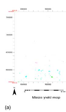
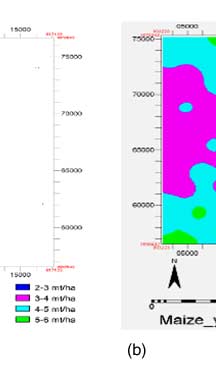
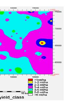
| Figure shows the maize yield map resulted from relationship between salinity and total dry mass. Maize yield estimated higher in depression and its periphery. Yield collected from the farmers are closely related with estimated yield. Generally, yield from farmers field varied from 4 to 6 mt/ha which correlate well with yield map obtained from the simulation. Farmers express yield in average that could not be used to validate the results. |
|
| Figure 2 : (a) Maize yield map, (b) Potential maize yield class |
|