home    land degradation    project outcome    Gallery Flooding Flood Hazard Assessment Pilot Area • The Pilot Areas • Climate • Cover factor (C) estimation • Digital terrain analysis • Relationship between soil properties • Relationship of soil properties with different land use/cover types Methodology • Methodologies • LISEM Results • Result Soil Properties and Land Use • Runoff rate for different land cover types • Model calibration and validation • Sensitivity analysis • Land use scenarios • Rainfall size scenarios • Flooding Scenario - 2 years return period • Flooding Scenario - 10 years return period • Flooding Scenario - 20 years return period • Flooding Scenario - 50 years return period • Summary tables for each flood characteristic • Flood hazard mapping • Conclusions and Recommendation Erosion Erosion Assessment Pilot Area • The Pilot Areas • Climate • Cover factor (C) estimation • Digital terrain analysis • Relationship between soil properties • Relationship of soil properties with different land use/cover types Methodology • Methodologies • Erosion Models Result • Results • C-Factor Mapping for erosion assessment • Soil erosion assessment • Assessment of land use/cover change effect on soil erosion • Assessing critical zones for ephemeral gully formation • Erosion Assessment by Different Models • The recommended erosion models • RMMF Landslide Case I • Landslide hazard assessment • The area (Pilot 3) • Landslide Mapping in Wang Chin using digital image analysis Techniques. • Results • Discussions Case II • Doi Ang Khang (Ang Khang) (Pilot area 4) • Landslide mapping in Ang Khang using aerial photos • Landslide Inventory Mapping • Landslide modelling and Susceptibility mapping • Landslide Susceptibility Maps from the three Scenarios (models) • Comparison between Ang Khang and Wang Chin (with respect to weights of evidence modelling using morphometric parameters) Salinization Case I • Pilot area II • Soil salinity • Salinization • Geomorphology • Soils • Geopedologic map • Results Case II • CASE II - The study of Yadav, R.D. (2005), • Methodology • Crop Simulation Model • PS 123 • Results • Mathematical (Regression) Model for Crop Yield Estimation • Conclusion Case III • Case III • Modeling Salinization • Geostatistics and Interpolation (GIS and Kriging) • Model Simulation and Prediction of Salinity • Simulated Depth to water table • Tenth Years Prediction • Twenty Years Prediction • Conclusion Runoff • Surface Runoff • Methodology • Modelling Runoff • Modelling Runoff Using Empirical Approach • Modelling runoff using the Semi-physical approach • Estimation with the Curve Number Method • Results and Discussion • Generation of Scenarios • Comparison of runoff rates with soil loss map • Conclusions • Presentation of papers based on project work at international • Workshop in Lomsak • Hua Hin seminar • Training of LDD staff • GIS and RS based predictive soil mapping • Soil erosion assessment • Landslide hazard assessment • Flood hazard assessment • Soil salinity study • List of completed MSc. 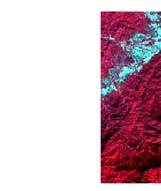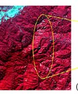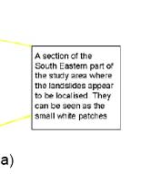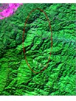theses on project RESULTS Only recent slides could be recognised by the digital image analysis technique and were thus classified as unvegetated scarps. The identified landslides were small in size, most of which were concentrated on the South Eastern side of the study area which runs parallel to the lateral/tributary valley. The Landslide inventory derived from aerial photo interpretation was used as the ground truth to test the accuracy of the landslide maps obtained from digital image analysis techniques. Results show that areas covered by landslides vary depending on the type of techniques used (Table 1). Areas under landslides were computed using histogram calculations. Histogram information reveals that NDVI is the technique with not only the least coverage (13.1 ha) in terms of area but also one with the least accuracy (18.88%). NDVI is a classification best designed for differentiating between land cover classes most especially between vegetation, water and bare soil (Sabins 1996). As a result it is too general and its ratios are only indicative and not specific. Table 1 : Results showing coverage of landslides by area using the different techniques Analysis Technicque Number of Pixels Area (m) Area (ha) NDVI 40427 131172 13.1 SAM 67756 271024 27.1 Maximum Likelihood (without Intensity Normalisation) ML 234578 938348 93.8 Maximum Likelihood (with Intensity Normalisation) NML 176620 706480 70.6 Digital Aerial photos Interpretation (Ortho photo) 40427 161708 16.2 Use of Maximum Likelihood Supervised Classification with Slope and Geology maps in Digital Image Analysis. This section involved the selection of bands which would result into the best classification results once compared with the landslide map from aerial photo interpretation. The selection helps the expert to different between the classes (or features) being classified since spectral characteristics of different features vary in the different bands (Lillesand, Kiefer et al. 2004). The selection of bands is also dependent on what purpose the classification is supposed to serve. This could be land use/ land cover or Geology or landslide mapping like in this study. Before this process was started, a Level 1B Geo- coded ASTER image was obtained and a sub set was created in an attempt to reduce the size of the image. Selection of band combinations for the map lists used in the training and classification phase. Bands 1, 2 and 3 were selected as the first band combination to establish how much could be obtained using the bands from VNIR region of the spectrum. The other band combinations were based on the correlation amongst the various bands of the ASTER image. The correlations were calculated using correlation matrices. When analyzing satellite data, the various spectral bands often show a degree of correlation (Lillesand, Kiefer et al. 2004). This means that when spectral values in one band are high the values in another band are expected to be high as well as discussed by (Richards 1993). He observed that plotting values from highly correlated bands in a feature space will result in an ellipsoid denoting that the two bands contain dependent information. From a set of highly correlated bands only one adds real value whilst the other ones may be derived or estimated (Richards 1993). Calculating a correlation matrix helps to detect the redundancy and identifies possible reductions in the number of bands to be used in a color composite. Correlation coefficients are normalized covariance values. A correlation coefficient ranges from - 1 to +1 (Lillesand, Kiefer et al. 2004). Diagonal elements are always 1. (Lillesand, Kiefer et al. 2004) noted that a correlation close to +1 indicates a direct relationship between two bands. They then suggested that if the reflectance of a pixel in one band is known, the reflectance of that pixel in the other band can be derived or estimated. A correlation close to -1 indicates an inverse relationship between the reflectance values of one band and the reflectance values in the other one(Lillesand, Kiefer et al. 2004). a) Bands 1,2 and 3 from the VNIR regions (RGB:321 respectively) Bands 1, 2 and 3 are the bands from the VNIR region of the spectrum. Figure 1 shows a false color composite made using these 3 bands. 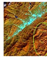The landslide results obtained from this map list are presented in Table 2 Figure 1 : Showing the color composites for Band Combinations 1,2,3 (a); Bands 2,3,4 (b) and Bands 1,3,7 (c), used in the Post processing phase Bands 2,3 and 4 from both VNIR and SWIR regions respectively To establish the correlation for the bands of the ASTER image used in this study, 4 bands were selected. These were bands 1, 2 and 3 of the Visible Near Infra red (VNIR) region and band 4 of the Short Wave Infra red (SWIR) region of the spectrum. The results of the correlation matrix are presented in Table 4.3. Bands 1 and 2 are highly correlated with a correlation coefficient of 0.95. The high correlation between bands 1 and 2 suggests that one of these bands could be removed from the band combination. In addition to this, band 1 has the highest correlation with the rest of the bands in this group in comparison to band 2. So band 1 was left out and band 2 was used. Therefore a map list of bands 2, 3 and 4 was created and used. Band 4 of the SWIR region was resampled to 15m resolution before the map list was created. 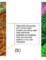Table 2 : Showing results of the Correlation Matrix for four band combinations used in this study Bands Band 1 Band 2 Band 3 Band 4 Band 7 Band 1 1.00 0.95 0.88 0.82 0.71 Band 2 0.95 1.00 0.72 0.78 0.80 Band 3 0.88 0.72 1.00 0.77 -0.01 Band 4 0.82 0.78 0.77 1.00 0.69 Band 7 0.78 0.63 1.00 0.69 1.00 The band combination (RGB: 432 respectively Figure 4.6b) was useful in visualisation of the Geology of the area. One type of Geology (Shale, Sandstone and Conglomerates) is prone to landslides (with respect to the study area). This band combination helped in identifying possible reasons for the localization of the landslides. In addition during the training phase, the bare land was clearly visible which helped in the reduction of errors during the training phase. Bands 7 (SWIR ), 3 and 1 from and VNIR regions (RGB:731 respectively Figure 4.6 c) Selection of these bands was based upon their correlation (Table 2). Although the correlations seem to be high, they are relatively lower than the correlations amongst the other bands ensuring a maximization of the spectral characteristics of the features shown on the image. The result is less overlap and clear differentiation between the classes during the training phase and classification. 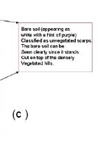Apart from the relatively lower correlation, this band combination gives a visualisation that is almost a true color composite. This is because vegetation is clearly visible as green (real color of healthy vegetation naturally), built up areas as purplish while the bare soil is clearly distinguished (area of focus). The clear visualisation reduces the error during the training phase since there is a clear distinction between built up areas and bare soil. Bands 1,2,3 (from VNIR region) and 4,5 and 6 (from SWIR region) Bands from the SWIR region were used to determine whether use of a SWIR region band would have any impact on the results of the classification. Thus results from the classifications of the above band combinations are presented in Table 2. After establishing the correlation amongst the various bands as indicated in Table 4.3, map lists for the band combinations were created. That is for the combination of Bands 1,2 &3, Bands 2,3 &4, Bands 1,3,&7 and Bands 1,2,3,4,5&6. A sample set then created for each of these map lists but the same domain was maintained and it contained three classes; bare soil, unvegetated scarps and others. The next phase was to train the data set for each of the map lists and then run the classification algorithm. The results were then post processed in an effort to improve the classification results and the accuracy. Table 3 : Showing results of the classification of the image using the selected band combination Band Combination Unvegetated Scarps (No. of Pixels) Percentage of Whole map (%) Number of Pixels of the whole image 123 2815755 4.49 62672550 234 1489696 2.38 62672550 731 6812782 10.87 62672550 123456 437189 0.70 62672550 Map (for testing accuracy) Number of Pixels Area (m2) Slide 01 52921 211684 The results in Table 3 indicate that band combination 1,3, & 7 has the highest percentage of pixels classified as unvegetated scarps and while band combination 1,2,3,4,5&6 indicates the least number of pixels classified as unvegetated scarps. Bands 1,2 & 7 seem to indicated (based on the results Table 3 that the presence of Band 7 improves on the classification results. This could be due to the fact that this band combination is good for visualtion and reduces the user’s error of accuracy during the training phase. References Sabins, F. ( 1996). Remote Sensing:principles and interpretation. New York:, W.H. Freeman and Company. Lillesand, M. T., W. R. Kiefer, et al. (2004). Remote Sensing and Image Interpretation. New York, John Wiley & Sons. Development of Methodologies for Land Degradation Assessment Applied to Land Use Planning in Thailand ^go to top